Noise Removal with Connected Components Analysis using GDAL and OpenCV

Introduction

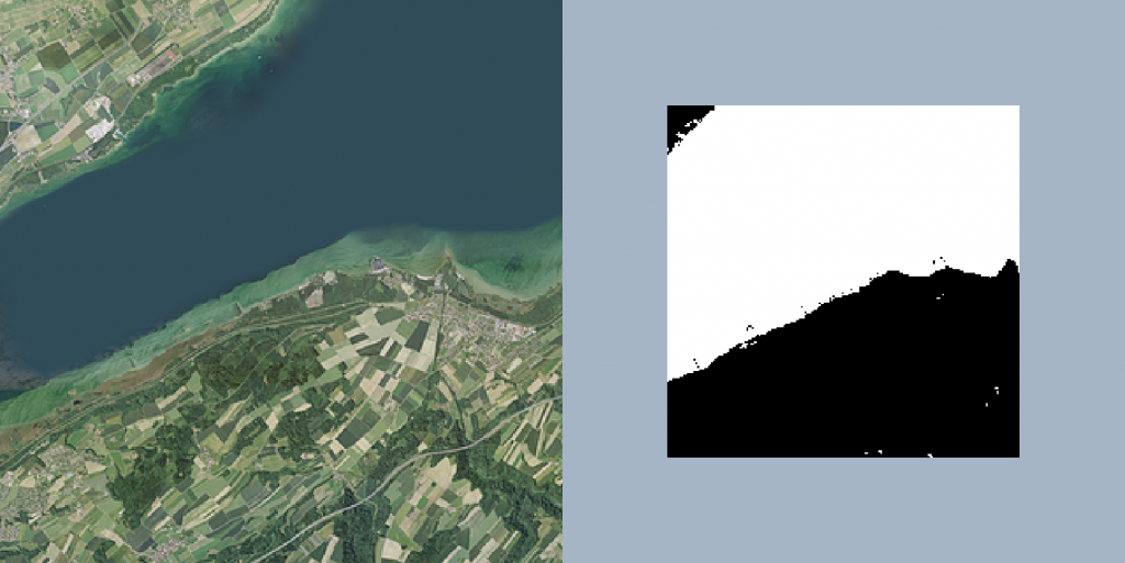
In a series of earlier posts, we have discussed how geospatial imagery can be segmented using a deep neural network. When applying such a trained model to imagery data, noise is a common and often not desirable phenomenon. Figure 1 depicts how such a segmentation result might look like, including a few white pixels afar from the central lake area. In this post, we are going to discuss how these can be removed with connected component analysis.

Connected Components Analysis

There are several ways how the noise depicted in Figure 1 can be removed. A straightforward approach would probably be morphological operators, e.g., by using a so-called “opening” operation. However, morphological operators have the disadvantage of changing the geometry of pixel clusters that are not considered as noise. An alternative to this is connected components analysis (CCA). In essence, CCA separates a binary image into areas (“components”) of connected pixels. For example, four white pixels forming a block and that are surrounded by black pixels would be considered a component. Gladly, libraries such as OpenCV can be used to perform CCA in an easy manner. The following code illustrates how CCA can be used to filter noise:

from osgeo import gdal
import cv2

# open the raster file
sample_dataset = gdal.Open("sample.tif")
sample_array = sample_dataset.ReadAsArray()

# calculate connected components
labels_count, labels, statistics, centroids  = cv2.connectedComponentsWithStats(sample_array, 4, cv2.CV_32S)

# define a threshold for pixel clusters
t = 10

# iterate over the labels
for idx in range(labels_count):
    mask = (labels == idx)
    
    # if the component is smaller than 10 pixels, change the cell values to 0
    if statistics[idx, 4] < t:
        sample_array[mask] = 0

    
# write the resulting raster to a file
driver = gdal.GetDriverByName("GTiff")
out_dataset = driver.Create("sample_removed_noise_cc.tif", sample_array.shape[1], sample_array.shape[0], 1, gdal.GDT_Byte, ['COMPRESS=LZW'])
out_dataset.SetGeoTransform(sample_dataset.GetGeoTransform())
out_dataset.SetProjection(sample_dataset.GetProjection())
out_dataset.GetRasterBand(1).WriteArray(sample_array)
out_dataset.FlushCache()
out_dataset = None

In lines 1 & 2 we are going to load the relevant libaries. In this case, only GDAL to load geospatial imagery and OpenCV to perform CCA. We are then loading the binary image as a numpy array on which we like to perform CCA (lines 5 & 6). Then, we already can apply CCA using OpenCV’s connectedComponentsWithStats() function (line 9). As a first argument, it takes the numpy array to work on, as a second argument it takes the connectivity (i.e., whether a a Moore or a Von Neumann neighborhood should be used) and as a last argument it takes a value to determine what data type the output should have. At the time of writing this is either a 32bit signed integer (as shown in the code) or a 16tbit unsigned integer. The method returns four variables. First, the number of found components (labels_count). Second, an array of the same shape as the input array (labels). Each pixel of labels holds a specific number determining to which component that pixel belongs. For example, all pixels labeled with the number 10 belong to the same component. Third, it returns a statistics array that holds additional information for each component (statistics) and fourth it returns an array that holds the centroid coordinates of each component (centroids). We then define a threshold t, which will later be used to filter components whose number of pixels falls below this value (line 12). Now, we can iterate over all the the found components (line 15). In each iteration, we create a boolean mask for each of the components by determining those pixels whose value corresponds to the current component number (line 16). We then can use the statistics information for the current component to get the area, i.e., the number of pixels. This information is given at the fourth position within that array. Positions zero to three define the bounding box of the component. We compare this value with the threshold we defined earlier. If the area of the compnent is smaller than the threshold, all of its pixels are set to zero (line 19), essentially removing the component (line 20). The result is depicted in Figure 2.

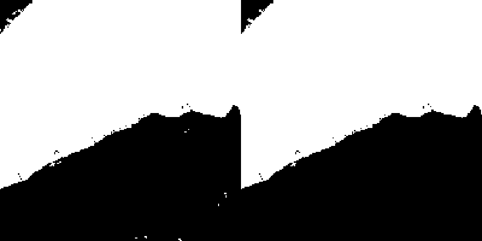
Figure 2: The original segmentation image (left) has been processed with Connected Components Analysis (CCA) to remove noise (right).

Finally, we create write the newly generated array to the disk (lines 24-30). If you are wondering what these lines mean, you can have a look at this blog post, where things are explained in greater detail.

Conclusion

In this post, we had a look at how Connected Components Analysis (CCA) can be used to remove noise from predictive results of segmentation models. OpenCV’s implementation of CCA can be used in a straightforward manner and integrates well with GDAL. In future posts, we may have a closer look at other functions from OpenCV and how they can be used in the context of geospatial analysis.