Semantic Segmentation of Geospatial Imagery with Deep Learning Part 6 – Model Inference and Evaluation

Introduction

In the previous post, we have successfully trained a model for lake segmentation. In this post, we are going to have a look at how its performance can be quantitatively and qualitatively assessed as well as how it can be used to generate lake segmentations for larger areas. We are going to have a look at how the model can be used to create predictions for a single SWISSIMAGE image and how misclassifications can be visualized. Finally, we are going to have a look at some common performance metrics useful for evaluating the model.

Visualizing Lake Predictions and Prediction Errors

Remember that we have divided our samples into three datasets, the training and validation datasets that are used during taining and a third dataset for testing. We are going to use this third testing dataset to make predictions and evaluate how well the model performs.

import numpy as np
import torch
import os
from osgeo import gdal
from sklearn import metrics


# load the model and set it to evaluation mode
unet = torch.load("./model.pth").to("cuda")
unet.eval()

# read all the SWISSIMAGE and lake mask images
swissimage_paths = "./samples/test_paths_images.txt"
mask_paths = "./samples/test_paths_masks.txt"

with open(swissimage_paths) as swissimages_file:
    swissimage_paths = swissimages_file.readlines()
    swissimages = [swissimage_path.rstrip() for swissimage_path in swissimage_paths]

with open(mask_paths) as mask_file:
    mask_paths = mask_file.readlines()
    masks = [mask_path.rstrip() for mask_path in mask_paths]

predictions = []
groundtruths = []

# prevent gradients to be calculated
with torch.no_grad():

    # iterate over all the training samples
    for i in range(len(swissimages)):
    
        # load the SWISSIMAGE and lake mask samples
        swissimage_path = swissimages[i]
        groundtruth_mask_path = masks[i]
        
        swissimage_dataset = gdal.Open(swissimage_path)
        swissimage_array = swissimage_dataset.ReadAsArray() / 255
        
        mask_dataset = gdal.Open(groundtruth_mask_path)
        mask_array = mask_dataset.ReadAsArray()

        swissimage_array_expanded = np.expand_dims(swissimage_array, 0)
        swissimage_tensor = torch.from_numpy(swissimage_array_expanded).float().to("cuda")
        
        
        # get the predicted mask of the model based on the SWISSIMAGE sample
        prediction_mask = unet(swissimage_tensor).squeeze()
        prediction_mask = torch.sigmoid(prediction_mask)
        prediction_mask = prediction_mask.cpu().numpy()
        
        
        # discretize the predictions by setting a threshold of 0.5
        prediction_mask = (prediction_mask > 0.5) * 255
        prediction_mask = prediction_mask.astype(np.uint8)
        
        
        # store the prediction result
        transform = mask_dataset.GetGeoTransform()
        projection = mask_dataset.GetProjection()
        
        driver = gdal.GetDriverByName("GTiff")
        out_dataset = driver.Create("./samples/prediction/" + groundtruth_mask_path.split("/")[-1], prediction_mask.shape[1], prediction_mask.shape[0], 1, gdal.GDT_Byte, ['COMPRESS=LZW'])
        out_dataset.SetGeoTransform(transform)
        out_dataset.SetProjection(projection)
        out_dataset.GetRasterBand(1).WriteArray(prediction_mask)
        out_dataset.FlushCache()
        out_dataset = None

        (...)

To use our model to make predictions, we are going to load our model and store it in video memory (lines 9 & 10). We are then loading the paths to our test dataset, i.e., for the SWISSIMAGE images and corresponding lake mask images (lines 13-22). Now that we have our datasets and the model in place, we disable gradient calculation for the model (line 28) and then iterate over all the SWISSIMAGE and lake mask images (lines 31-35). Each SWISSIMAGE image is normalized (line 38) and a dummy dimension is added to conform to the format required by PyTorch (line 43). Finally, the image is transformed into a PyTorch tensor and sent to video memory (line 44). The tensor is then passed to the U-Net model, which predicts a lake mask for this image (line 48). In the same line, any non-required dimensions are removed via the .squeeze() method. The result is passed through a sigmoid function to be mapped to the range [0, 1] and finally stored as a numpy array (lines 49 & 50). The predictions are discretized by determining whether the predicted value is larger than 0.5 or not (line 54). All values larger than 0.5 are stored as the value 255, which makes visualizing the data easier. All other values are stored as the value 0. Casting the array type to uint8 makes the dataset leaner (line 55). The resulting prediction mask is then stored to disk (lines 62-68). Let’s have a look at the second part of the script:

        (...)

        # convert the prediction mask and the groundtruth mask into a boolean array
        prediction_mask_bool = prediction_mask == 255
        groundtruth_mask_bool = mask_array == 255
        
        
        # keep track of the predictions as 1D arrays
        predictions += list(prediction_mask_bool.flatten())
        groundtruths += list(groundtruth_mask_bool.flatten())
        
        
        # calculate true positives (tp), true negatives (tn), false positives (fp) and false negatives (fn)
        tp = prediction_mask_bool & groundtruth_mask_bool
        tn = ~prediction_mask_bool & ~groundtruth_mask_bool
        fp = prediction_mask_bool & ~groundtruth_mask_bool
        fn = ~prediction_mask_bool & groundtruth_mask_bool
        
        
        # store the the metrics in an additional image
        error_image = np.zeros(shape=(prediction_mask.shape[0], prediction_mask.shape[1]), dtype=np.uint8)

        error_image[tp] = 0
        error_image[tn] = 1
        error_image[fp] = 2
        error_image[fn] = 3
        
        
        # write the error image to disk
        driver = gdal.GetDriverByName("GTiff")
        out_dataset = driver.Create("./samples/prediction/" + groundtruth_mask_path.split("/")[-1][:-4] + "_errors.tif", prediction_mask.shape[1], prediction_mask.shape[0], 1, gdal.GDT_Byte, ['COMPRESS=LZW'])
        out_dataset.SetGeoTransform(transform)
        out_dataset.SetProjection(projection)
        out_dataset.GetRasterBand(1).WriteArray(error_image)
        out_dataset.FlushCache()
        out_dataset = None

In the same loop in which we iterate over the single samples, we can determine for which image pixels correct or wrong predictions were made by the model. To do this, we are first creating boolean masks based on both, the predicted mask and the groundtruth mask (lines 4 & 5). Note that we are also storing both predictions as 1-dimensional arrays to later calculate more advanced performance metrics (lines 9 & 10). Based on the boolean arrays, we can determine four different scenarios:

• The pixel has been predicted as lake and the groundtruth array classifies that pixel as lake (true positive)
• The pixel has been predicted not to be a lake and also the groundtruth array classifies that pixel not as a lake (true negative)
• The pixel has been predicted to be a lake, but the groundtruth array classifies the pixel to be no lake (false positive)
• The pixel has not been predicted to be a lake, but the groundtruth array classifies the pixel not to be a lake (false negative)

These are being calculated in lines 14-17. We then create a new array, which can be used to hold these errors (line 21). Each cell of this array will be assigned a number from 0 to 3, depending on which case applies to the respective pixel (lines 23-26). Finally, we write this error image to disk (lines 30-36). An example of how the error mask can be visualized alongside the predicted and the groundtruth data can be found in Figure 1.

Finally, we can also calculate some global performance metrics, which provide complementary information about the quality of the model:

# calculate different metrics to determine the performance of the network
accuracy = metrics.accuracy_score(predictions, groundtruths)
print("accuracy", accuracy)

precision = metrics.precision_score(predictions, groundtruths)
print("precision", precision)

recall = metrics.recall_score(predictions, groundtruths)
print("recall", recall)

f1 = metrics.f1_score(predictions, groundtruths)
print("f1", f1)

jaccard = metrics.jaccard_score(predictions, groundtruths)
print("jaccard", jaccard)

Here, we are passing the predictions and groundtruth lists, which have been previously assembled, to boiler-plate functions provided by scikit-learn. Specifically, we are calculating the metrics accuracy, precision, recall, f1 and jaccard. Typically, a value close to 1 is considered good while lower values are considered worse. For example, the following metrics were obtained for one of the trained models:

• accuracy: 0.99581
• precision: 0.8671
• recall: 0.98930
• f1: 0.92421
• jaccard: 0.85910

Detailed information about these metrics and more metrics to explore can be found in the scikit-learn documentation. Note that these metrics likely differ each time a new model is trained due to randomization in the training procedure.

Making Large-scale Predictions

We have now seen how predictions can be made for single tiles and how performance metrics can be calculated. In practice, however, we would often like to process a larger image. The easiest way to accomplish this is to subdivide the larger image into single tiles, process each tile separately and finally stitch them together again. The following code can be used for this purpose:

import matplotlib.pyplot as plt
import numpy as np
import torch
import os
from osgeo import gdal
from sklearn import metrics

# load the model
unet = torch.load("./model.pth").to("cuda")
unet.eval()


# define the extents of the samples
sample_core = 100
sample_padding = 60
sample_extent = 2 * (sample_core + sample_padding)
sample_extent_core = 2 * sample_core
sample_extent_padding = 2 * sample_padding


# load the SWISSIMAGE mosaic
swissimage_dataset = gdal.Open("./swissimage/SI25-2012-2013-2014.tif")
swissimage_array = swissimage_dataset.ReadAsArray() / 255


# create an empty array to store the predictions in
result_array = np.zeros(shape=(swissimage_array.shape[1], swissimage_array.shape[2]))


# calculate the number of samples for the horizontal and vertical dimensions
vertical = swissimage_array.shape[1]
horizontal = swissimage_array.shape[2]

num_vertical = int((vertical - sample_extent) / sample_extent_core)
num_horizontal = int((horizontal - sample_extent) / sample_extent_core)


# disable gradient calculation and iterate over the samples to process
with torch.no_grad():
    for v_idx in range(num_vertical):
        for h_idx in range(num_horizontal):
            print(v_idx, num_vertical, h_idx, num_horizontal)
            
            
            # take the SWISSIMAGE subset and transform it into a PyTorch-compatible format
            swissimage_subset = swissimage_array[:,v_idx * sample_extent_core: v_idx * sample_extent_core + sample_extent, h_idx * sample_extent_core: h_idx * sample_extent_core + sample_extent]
            swissimage_subset_expanded = np.expand_dims(swissimage_subset, 0)
            swissimage_tensor = torch.from_numpy(swissimage_subset_expanded).float().to("cuda")
            
            
            # let the model make the prediction
            prediction_mask = unet(swissimage_tensor).squeeze()
            prediction_mask = torch.sigmoid(prediction_mask)
            prediction_mask = prediction_mask.cpu().numpy()
            prediction_mask = (prediction_mask > 0.5) * 255
            prediction_mask = prediction_mask.astype(np.uint8)

            
            # store the result
            result_array[v_idx * sample_extent_core + sample_padding: v_idx * sample_extent_core + sample_padding + sample_extent_core, h_idx * sample_extent_core + sample_padding: h_idx * sample_extent_core + sample_padding + sample_extent_core] = prediction_mask


# write the predictions to disk
driver = gdal.GetDriverByName("GTiff")
out_dataset = driver.Create("./sheet/predictions.tif", result_array.shape[1], result_array.shape[0], 1, gdal.GDT_Byte, ['COMPRESS=LZW'])
out_dataset.SetGeoTransform(swissimage_dataset.GetGeoTransform())
out_dataset.SetProjection(swissimage_dataset.GetProjection())
out_dataset.GetRasterBand(1).WriteArray(result_array)
out_dataset.FlushCache()
out_dataset = None

Most of the code should look familiar. We are first loading the model (lines 9 & 10), and then define some useful information about the possible extents of the samples (lines 14-18). We then load the whole SWISSIMAGE dataset and normalize it (lines 22 & 23). We then create an empty array to store the results in (line 27). The number of tiles in the vertical and the horizontal directions are calculated (lines 34 & 35) and used to iterate over the whole image (lines 40 & 41). In that loop, we first crop a tile from the SWISSIMAGE image and transform it to be readable by PyTorch (lines 46-48). We then again let the model predict the lake mask (lines 52-56) and store the result in the array we created before (line 60). Finally, we write the whole array to disk (lines 64-70). One possible result of this procedure is shown in Figure 2.

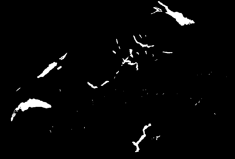
As can be seen from Figure 2, the model seems to perform reasonably well, although several artefacts (especially false negatives) in the area of lake Geneva are obvious. The model could certainly be further fine-tuned in several ways: the lake dataset could be manually improved to better match the underlying imagery and it the training dataset as a whole could be augmented (i.e., rotated, mirrored or even distorted), which would yield a larger overall dataset for training. One could also try different metaparameters by adjusting the learning rate, the number of layers, different activation functions, etc. Potentially, one could even test an entirely different segmentation architecture. All of these possibilities, however, are out of scope of this blog post series. In any case, I hope that this series provided some useful information about how the to set up a deep learning pipeline to process geospatial imagery.

Conclusion

In this post, we have explored ways of how the trained model can be applied to existing data, i.e., by applying it to the samples of the test dataset as well as to the whole SWISSIMAGE dataset. We also have briefly investigated how prediction errors can be visualized and how global performance metrics can be calculated. The series gave a somewhat complete picture about how a deep learning model can be trained to process geospatial imagery. As the pipeline is somewhat generically applicable, I am hoping that the series provided enough information for the reader to set up similar pipelines for other use cases.