Introduction
In the previous post, we have set up our working environment. In this blog post, we are going to have a look at from where we can obtain suitable training datasets. Training a deep learning model is only possible if a large volume of suitable data is available. Thankfully, many governments have started to publish their geodata online for everyone to explore and use. As we are going to train a deep learning model that is supposed to determine whether a pixel on an image is part of a lake or not, we require two datasets: the aerial imagery raster files from which the features should be detected (typically georeferenced RGB images) and the groundtruth data, i.e., in the form of binary image files that hold information for each pixel whether it belongs to a lake or not. This is commonly encoded as a number, i.e., 1 for “here is a lake” and 0 for “here is no lake”.
Data Download
For the scope of this series of blog posts, we are going to use data by Swisstopo, the federal surveying and mapping agency of Switzerland. Specifically, we are going to use the “SWISSIMAGE” dataset with a resolution of 25cm and lake vector data from the “Swiss Map Vector” (SMV) dataset. The “SWISSIMAGE” dataset can be directly downloaded from here for the whole area of Switzerland as one file. The SMV dataset is available for different regions of Switzerland as single tiles that later need to be merged. To download these tiles, one can go to the download site and chooses “Entire data set” as the “Selection mode”. Then, one can click on the “Search” button. After a short while, the links to the single tiles can be downloaded as a CSV file when clicking on “Export all links”. The file can also be downloaded directly from here:
Now, downloading each of the listed files manually is cumbersome. However, each of these files can also be downloaded via a script:
import requests

# open the csv file that contains the links
with open("ch.swisstopo.swiss-map-vector25-JoxjV3rw.csv", "r") as csv_file:
    # iterate over each entry of the csv file
    for line in csv_file:
        stripped_line = line.strip()
        name = stripped_line.split("/")[-1]
        print(stripped_line)
        # download the data at the URL and store it to the disk
        r = requests.get(stripped_line, allow_redirects=True)
        open("./smv/" + name, 'wb').write(r.content)
The script imports the requests library that can be used to download files (line 1). It then opens the CSV file (line 4) and iterates over each entry (line 6). The end-of-line character is removed from the entry (line 7) and the content is downloaded and stored in a directory “smv” under the name corresponding name (lines 11 and 12).
Finally, we are also going to need the swissBoundaries3D dataset. It can be obtained from here. Specifically, we are going to use the archive swissboundaries3d_2022-05_2056_5728.shp.zip. Within this archive, we will make use of the file swissBOUNDARIES3D_1_3_TLM_LANDESGEBIET.shp, which contains the area of Switzerland as a polygon (and some other regions).
Data Preprocessing
The SWISSIMAGE file is already in a suitable format and does not require any special processing. However, the lake data is stored as vector layers in separate geopackage databases. This format is not directly suitable for deep learning applications. To make it usable, we first need to create a single vector layer containing all the lakes, and second, we need to rasterize this merged lake dataset.
To create a single layer that comprises all the lakes, we first need to extract the single zip files, which can be conveniently done with the windows explorer, for example. Once unpacked, the following script can be used to assemble a single lakes vector file:
import glob, os.path
import fiona, fiona.crs
from shapely.geometry import shape

# find all files that end with gpkg, i.e., that are geopackages
geopackage_paths = glob.glob("smv/**/**/*.gpkg", recursive=True)

# define a schema for the lakes to be stored in
schema = { 'geometry': 'Polygon', 'properties': {}}
lakes = fiona.open("lakes/lakes.shp", 'w', driver="ESRI Shapefile", schema=schema, crs=fiona.crs.from_epsg(2056))

counter = 0
num_paths = len(geopackage_paths)

# iterate over all the found geopackage paths
for geopackage_path in geopackage_paths:
    if counter % 10 == 0:
        print(str(counter) + "/" + str(num_paths))
    counter += 1

    # open the geopackage layer if the path points to a file
    if os.path.isfile(geopackage_path):
        with fiona.open(geopackage_path, layer="T56_DKM25_GEWAESSER_PLY") as layer:
            # iterate over all features in the water bodies layer
            for feature in layer:
                lake_geometry = shape(feature['geometry'])
                # store all geometries that are of type "See", i.e., lake
                if feature['properties']["OBJEKTART"] == "See" and (lake_geometry.type == "Polygon" or lake_geometry.type == "MultiPolygon"):
                    lakes.write({'geometry': feature["geometry"], 'properties': {}})
The script first recursively searches for all paths that end with “.gpkg” in the directory where we unpacked the geopackages (line 6). It then defines a schema and storage location of the file to which all the lakes should be written to (lines 9 & 10). It iterates over all found paths (line 16) and opens all found geopackage files (lines 22 & 23). Note that some directory names might also end with “.gpkg”, which need to be skipped (line 22). The used layer to open the geopackage is named “T56_DKM25_GEWAESSER_PLY”, which contains several types of hydrological features. The script then iterates over all features within that layer and stores their geometry only if they are of type “See”, i.e., if they are a lake, and if their geometry is of type “Polygon” or “MultiPolygon” (lines 25-29).
The result is a shapefile lakes.shp that contains all the lakes that were found. The next step is to rasterize these lakes. It is important that the resulting raster file has the exact same extent and resolution of the SWISSIMAGE file. The following script can be used for this purpose:
from osgeo import gdal
from osgeo import osr
from osgeo import ogr


# open lakes.shp shapefile and the swissimage geotiff
vector_path = './lakes/lakes.shp'
raster_path = './swissimage/SI25-2012-2013-2014.tif'

vector_map = ogr.Open(vector_path)
raster_map = gdal.Open(raster_path)

layer = vector_map.GetLayer()
geotransform = raster_map.GetGeoTransform()
projection = raster_map.GetProjection()


# define the output raster
out_path = './lakes/rasterized_lakes.tif'
driver = gdal.GetDriverByName("GTiff")
rasterization_dataset = driver.Create(out_path, raster_map.RasterXSize, raster_map.RasterYSize, 1, gdal.GDT_Byte)

rasterization_dataset.SetGeoTransform(geotransform)
rasterization_dataset.SetProjection(projection)


# use the RasterizeLayer method to rasterize the layer
gdal.RasterizeLayer(rasterization_dataset, [1], layer)

# clean up
rasterization_dataset.FlushCache()
rasterization_dataset = None
raster_map = None
First, we are opening the lakes.shp shapefile and the SWISSIMAGE geotiff (lines 7-11). From the lakes.shp, we take the layer, which contains all the features, and from SWISSIMAGE, we take the geotransform and the projection (lines 13-15). We then create a new dataset to which the lake features should be rasterized (lines 19-21). It has the same dimensions (RasterXSize, RasterYSize) as the SWISSIMAGE file, has 1 channel and is of type Byte. This datatype is sufficient, because it will only contain the value 0 for pixels where no lake is located and the value 1 for pixels where a lake is located. Furthermore, the geotransform and projection of the SWISSIMAGE geotiff are assigned to the newly created raster to ensure that they align geospatially (lines 23 and 24). The actual rasterization of the lakes is carried out in line 28 using the RasterizeLayer method provided by GDAL.
Conclusion
The three datasets, the SWISSIMAGE geotiff, the rasterized lakes geotiff, as well as the swissboundaries shapefile have been assembled. Figure 1 shows these three datasets. It is important to note that the swissboundaries nearly perfectly delineate the border of Switzerland. These three datasets form the building blocks to generate samples from which the deep learning model can be trained. We are going to have a closer look at this in the next blog post of this series.
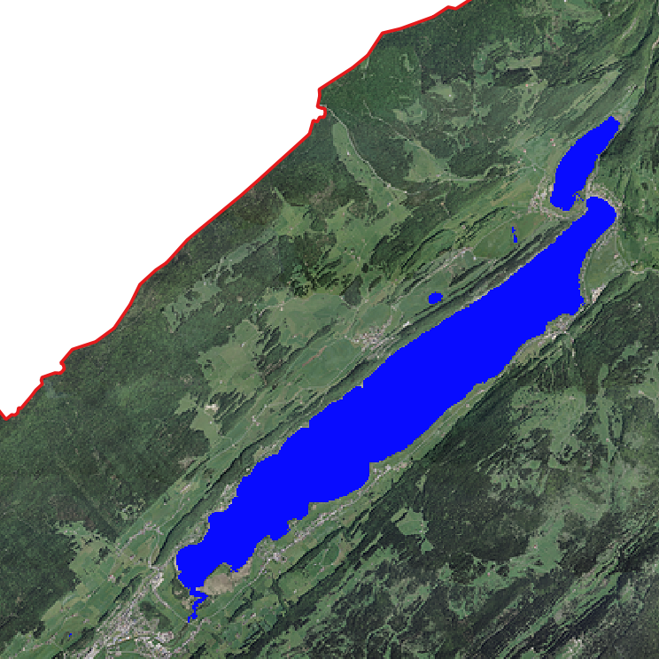
Figure 1: swissboundaries (red) and rasterized lake pixels (blue) superimposed on SWISSIMAGE.