Semantic Segmentation of Geospatial Imagery with Deep Learning Part 3 – Training Samples

Introduction

In the previous post of this series, we have acquired the relevant datasets and transformed the lake vector dataset into a raster file that aligns with the SWISSIMAGE dataset. In this blog post, we are going to use these datasets to create image samples that can be read by the deep learning model we are going to train.

Training Sample Characteristics

The segmentation model we are going to train is based on the so-called U-Net architecture. Originally proposed to carry out segmentation on biomedical images, it has been proven to be generically applicable to many image-based segmentation tasks. A detailed discussion about its functionality will be given in the next blog post. At the moment, it is important to understand that its input will be a large number of image crops from the SWISSIMAGE geotiff along with corresponding image crops from the geotiff of rasterized lakes. Due to memory limitations, it is not possible to read the whole SWISSIMAGE and rasterized lake geotiffs in one go. Hence, they need to be cropped. In addition, the sizes of the SWISSIMAGE crops should be chosen to be somewhat larger than the image crops which represent the segmentations of lake pixels and non-lake pixels. The reason for this lies in the idea that for a given SWISSIMAGE image, there is not enough context information available at the borders to determine whether a pixel belongs to a lake or not. For example, a single dark blue pixel at the border could also be part of shade, a roof or could simply be a color artefact. Reasonable accuracy can only be obtained for the innermost pixels. For the given setup, we choose the SWISSIMAGE image crops to have an extent of 320 pixels x 320 pixels (or 8000 meters x 8000 meters) and the target segmentation image crops to have an extent of 200 pixels x 200 pixels (or 5000 meters x 5000 meters).

Generation of Sample Locations

There are several ways of how geospatial imagery can be sampled and transformed to be used in deep learning models. A straightforward approach would be to read the image files as NumPy arrays and to slice them in regular intervals according to the sample dimensions. This would also require to check each sample for null values and to discard them if any are found as this might cause issues during training. However, this approach somewhat limits the control about where exactly the images are placed and potentially wastes locations where only few null values are present but the whole sample is discarded nontheless.

A somewhat more flexible way of how to determine where to place samples is by first creating a point vector layer in which each point represents a sample location. The points in this vector layer can be investigated and potentially modified in a GIS to better exploit the available data. The following script can be used to create such a point grid:

import shapely, fiona, fiona.crs
from osgeo import gdal
from shapely.geometry import Point, mapping, shape, CAP_STYLE
import math

# define sample size in pixel
sample_core = 100
sample_padding = 60

rasterized_path = "./lakes/rasterized_lakes.tif"
rasterized_dataset = gdal.Open(rasterized_path)


# get georeferencing and extent information
geot = rasterized_dataset.GetGeoTransform()
geoproj = rasterized_dataset.GetProjection()
extent_x = rasterized_dataset.RasterXSize
extent_y = rasterized_dataset.RasterYSize


# determine the extent of the raster
resolution_x = geot[1]
resolution_y = geot[5]
left = geot[0]
top = geot[3]

extent_x_geo = extent_x * resolution_x
extent_y_geo = extent_y * -resolution_y


# define sample size in meters
sample_core_geo = sample_core * resolution_x
sample_padding_geo = sample_padding * resolution_x

num_samples_x = int(extent_x_geo / (2 * sample_core_geo))
num_samples_y = int(extent_y_geo / (2 * sample_core_geo))


print("number of samples in the x direction:", num_samples_x)
print("number of samples in the y direction:", num_samples_y)


# the samples are stored in the Shapefile sample_points.shp
schema = { 'geometry': 'Point', 'properties': {}}
sample_points = fiona.open("./samples/sample_points.shp", 'w', driver="ESRI Shapefile", schema=schema, crs=fiona.crs.from_epsg(2056))


# the boundary of Switzerland is being loaded to remove those points that overlap with null values
extent_ch = fiona.open("./swissboundaries/swissBOUNDARIES3D_1_3_TLM_LANDESGEBIET.shp")
extent_ch_geom = shape(extent_ch[0]["geometry"])


# traverse the extent to create the point grid
for x_idx in range(num_samples_x):
    x_geo = left + x_idx * 2 * sample_core_geo
    for y_idx in range(num_samples_y):
        y_geo = top - y_idx * 2 * sample_core_geo
        
        point = Point(x_geo, y_geo)
        
        # check if the point falls within the boundaries of Switzerland
        if extent_ch_geom.contains(point.buffer(sample_core_geo + sample_padding_geo, cap_style=CAP_STYLE.square)):
            sample_points.write({'geometry': mapping(point), 'properties': {}})
        
        
sample_points.close()
extent_ch.close()

Most of the content of this script should be self-explanatory. First, the dimenions of the samples are defined (lines 7 & 8). Then, the geotiff with the rasterized lakes is being loaded from which different types of metadata are being retrieved (lines 10-25). Based on these information, the extent of the raster file is being calculated (lines 27 & 28) and the sample size in geocoordinates is being calculated (lines 32 & 33). Finally, the number of samples in the horizontal direction and the vertical direction are determined (lines 35 & 36). We create a new schema and file to store the sample points (lines 44 & 45). In addition, we load the extent of Switzerland which can be used as that area in which sample points are allowed to be placed (lines 49 & 50). We iterate over all the samples in both directions and calculate the sample point coordinates (lines 54-57). Based on these coordinates, a new sample point is being created (line 59). To be sure that the sample point lies entirely within the boundaries (and hence does not contain any null values), it is first being buffered according to the sample extent using a square buffer. The resulting geometry corresponds to the area that would be cropped and used for training the model. If this geometry exceeds the valid area of Switzerland, it will not be used as a training sample, because it would contain invalid values (lines 62 & 63). Finally, we are closing any opened datasets (lines 66 & 67).

Visualization and Manual Adjustment of Sample Locations

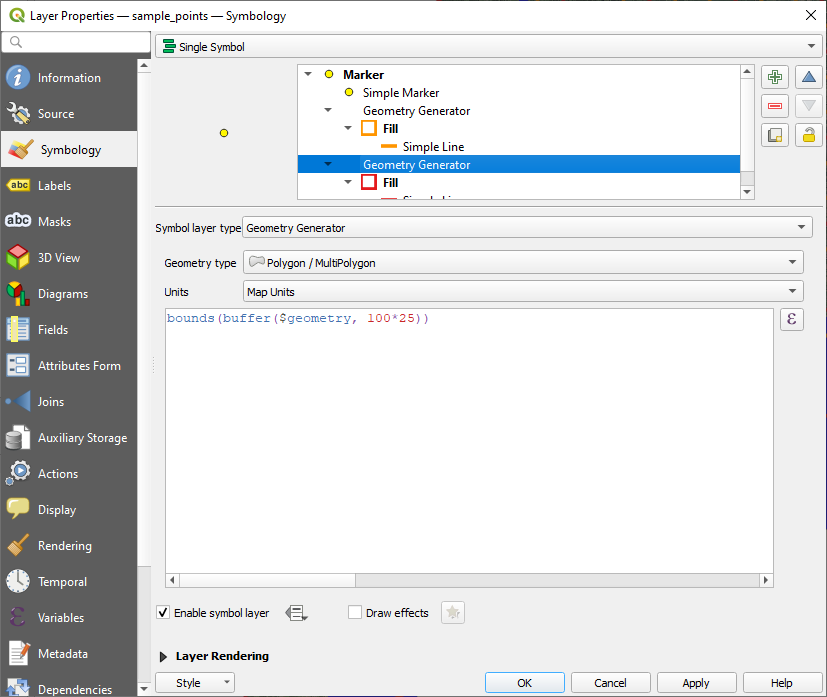
Now we have generated a first set of samples from which we are going to extract image crops for training. However, in many cases it can be beneficial to manually adjust these samples in order to better exploit the underlying datasets. To get a better idea about where the sample locations have been generated, it is helpful to visualize them. However, single point symbols are not sufficient to understand the area these samples are covering. Using QGIS it is possible to define custom symbols that transform single points into other geometries that are then being depicted. To achieve this, we are going to use geometry generators. In the “symbolization” properties of the point symbols, we are going to create two new geometry generators, one for each of the different crop sizes. The first geometry generator will be provided with the following expression:

bounds(buffer($geometry, 100*25))

Here, 100 is the extent of the inner crop area for which a segmentation is going to be made and 25 is the resolution, i.e., in meters per pixel. The second geometry generator will be provided with a slightly different expression:

bounds(buffer($geometry, 160*25))

Here, 160 represents the larger extent which will be analyzed to come up with the segmentation of the inner area. Figure 1 shows how the final symbolization setup looks like. The resulting point representations are depicted in Figure 2.

As it can be seen from the left side of Figure 2 , there are quite some areas that are not being properly sampled, because points created in a regular grid would overlap with the boundary and hence would contain null values. However, we can use QGIS efficiently to add more points that cover these locations. This might lead to larger overlaps, but in practice this is rarely an issue as long as it is not overdone. For example, lake Geneva does not contain many samples, so we added a few there to better exploit the available data (Figure 2 right).

Cropping

Now that we have properly put together all the necessary components, all that is left to do is to automatically extract the image crops:

import numpy as np
from osgeo import gdal
import fiona
import random

# read relevant raster datasets
lake_mask_path = "./lakes/rasterized_lakes.tif"
swissimage_path = "./swissimage/SI25-2012-2013-2014.tif"

sample_points = fiona.open("./samples/sample_points.shp")
lake_mask = gdal.Open(lake_mask_path)
swissimage = gdal.Open(swissimage_path)

# define the crop extents
sample_core = 100
sample_padding = 60
res = swissimage.GetGeoTransform()[1]

offset_swissimage = (sample_core + sample_padding) * res
offset_lake_mask = sample_core * res


point_counter = 0

base_path = "samples/"
mask_paths_file = open(base_path + "/mask_paths.txt", "w")
swissimage_paths_file = open(base_path + "/swissimage_paths.txt", "w")

# iterate over all the points
for point in sample_points:
    # write the locations of the cropped training images
    swissimage_sample_path = "./samples/swissimage/" + str(point_counter).zfill(4) + ".tif"
    swissimage_paths_file.write(swissimage_sample_path)
    swissimage_paths_file.write("\n")
    
    mask_sample_path = "./samples/mask/" + str(point_counter).zfill(4) + ".tif"
    mask_paths_file.write(mask_sample_path)
    mask_paths_file.write("\n")
    
    point_counter += 1
    
    if point_counter % 20 == 0:
        print(str(point_counter) + "/" + str(len(sample_points)))
    
    # retrieve the point coordinates
    x_coord = int(point["geometry"]["coordinates"][0])
    y_coord = int(point["geometry"]["coordinates"][1])
    
    # calculate the crop extent of swissimage
    ulx_swissimage = x_coord - offset_swissimage
    uly_swissimage = y_coord + offset_swissimage
    lrx_swissimage = x_coord + offset_swissimage
    lry_swissimage = y_coord - offset_swissimage
    
    gdal.Translate(swissimage_sample_path, swissimage_path, format='GTiff', options="-co TFW=yes -projwin " + str(ulx_swissimage) + " " + str(uly_swissimage) + " " + str(lrx_swissimage) + " " + str(lry_swissimage))

    # calculate the crop extent for the lakes
    ulx_lake_mask = x_coord - offset_lake_mask
    uly_lake_mask = y_coord + offset_lake_mask
    lrx_lake_mask = x_coord + offset_lake_mask
    lry_lake_mask = y_coord - offset_lake_mask
    
    gdal.Translate(mask_sample_path, lake_mask_path, format='GTiff', options="-co TFW=yes -projwin " + str(ulx_lake_mask) + " " + str(uly_lake_mask) + " " + str(lrx_lake_mask) + " " + str(lry_lake_mask))
    

# close the datasets    
mask_paths_file.close()
swissimage_paths_file.close()

We are first reading the necessary raster files (lines 7-12) and then define the extents that should be cropped (lines 15-20). We are creating two text files, which hold the relative paths to the samples we are using for extraction (lines 25-27). The extraction is being performed in lines 32-38 when iterating over all the points (line 30). Based on the x- and y-coordinates of the sample point (lines 46 & 47), the coordinates of the area to be extracted are being calculated for the SWISSIMAGE crops (lines 50-53) and for the lake raster files (lines 58-61). The actual cropping procedure is being carried out by the Translate method of GDAL, which takes the calculated offsets and writes the results as geotiffs (lines 55 & 63). Finally, the datasets are being closed (lines 67 & 68). An example of a cropped tuple of images is shown in Figure 3.

Conclusion

In this post, we have defined the locations from where the SWISSIMAGE and lake raster files should be sampled and have carried out a cropping procedure to build up the datasets for the model to be trained. Visualizing the sample points via QGIS can help assessing their coverage and at the same time allows to modify their locations to better cover the available datasets.